Mars in 3D! A Beginner’s Guide to 3D Modeling the Martian Terrain

3D modeling is a fun and easy way to engage in current NASA missions, though relatively few have tapped into its full potential. This blog guides readers through the step-by-step process used by the Mastcam-Z subteam at Cornell University to create structure-from-motion (SfM) models of the Martian terrain in hopes of increasing engagement and accessibility to groundbreaking science techniques for all. Though this tutorial focuses on modeling Martian features, please note the same process is applicable to any scientific, artistic, and recreational projects.

This tutorial will model the first abrasion patch made by Perseverance Rover: the Rubion Abrasion. The rover cuts away the top few millimeters of a rock’s rough surface using a rotating flat drill bit to expose a flat, unweathered surface in a circle of 5 cm in diameter. The rover’s WATSON camera then captures images of this patch from multiple angles to maximize the measurements our Mars2020 mission team can do back here on Earth. The surface of the Rubion Abrasion, however, was a bit too bumpy and was thus deemed unfit for proximity-based measurements. In creating a 3D model of this abrasion site, we can examine the site for ourselves to find irregularities that would have otherwise gone unnoticed.

Part I: Data Collection

1. Gathering the Images

To gather the images needed for modeling the Rubion Abrasion path, we turn to NASA’s official Mars2020 Mission website to find raw images by Perseverance Rover. Using the site’s filter feature, set the range to only target those images taken by Perseverance’s SHERLOC-WATSON instrument between sols 160 and 161 in order from oldest to newest. (See Figure 1)

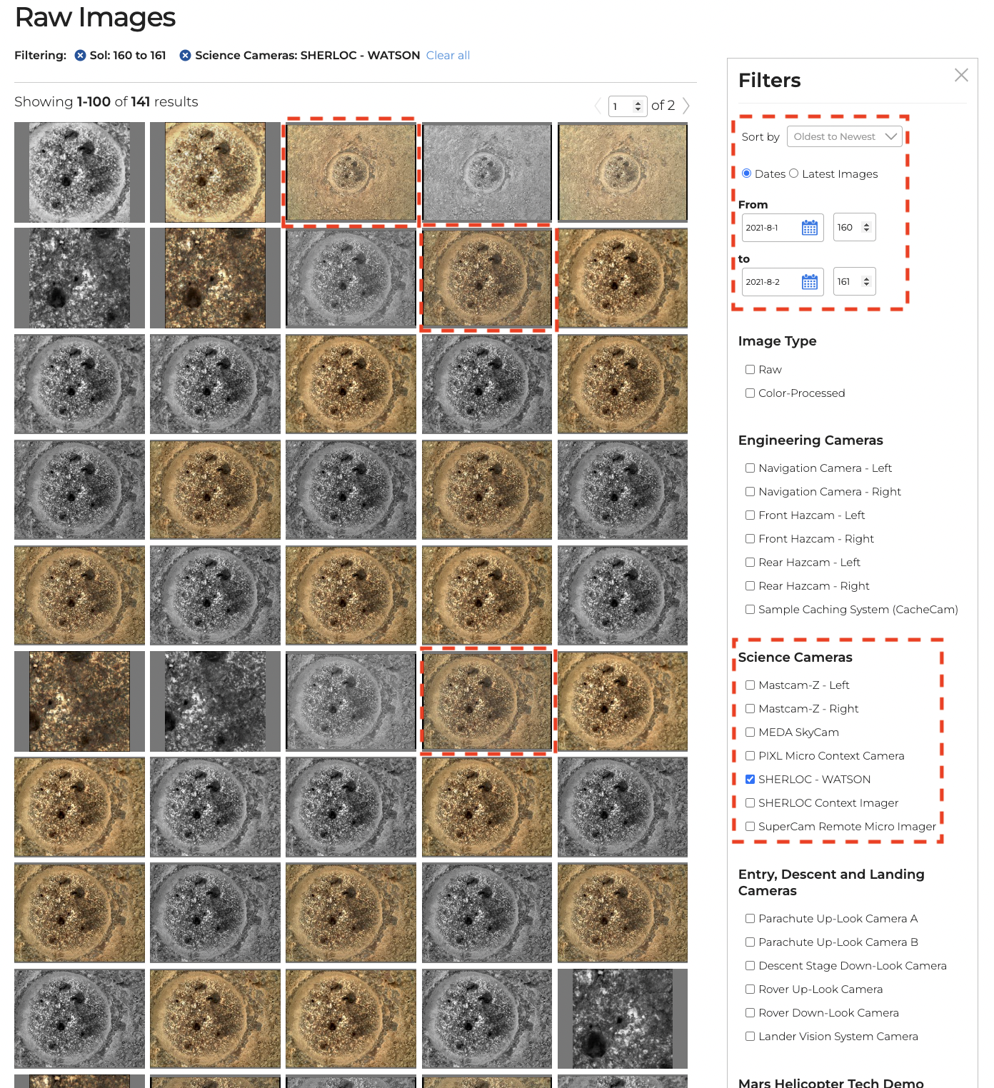Figure 1 Tips & Tricks: Downloading all files within this tutorial to the same folder on your device will make locating them a lot easier when uploading them to Agisoft Metashape.

Once filtered, download the first full frame colored image that follows each series of greyscale and extreme focus image pairs. These images should each have a small, black frame and may continue on page 2. In filtering these images, we now have a total of seven images from this specific abrasion site to download for our model.

For convenience, all data used throughout this tutorial can be downloaded from this “Mars in 3D Tutorial Toolkit”; however, we recommend following the process detailed above since it is applicable to all future models.

Part II: Creating a Model in Agisoft Metashape

To download the latest version of Agisoft Metashape, follow the instructions outlined on Agisoft’s installation webpage. By navigating the site, new users can find tutorials, tips, user manuals, and solutions to common errors such as this tutorial that covers these same basics. Please note this tutorial uses Agisoft Metashaper Pro 1.8.2, but we recommend either downloading the latest version of the software or taking advantage of Agisoft’s 30-day free trial to gain access to new features and avoid any bugs.

1. Importing Images to Agisoft Metashape

Upon starting Metashape, add the seven WATSON images by either double-clicking “Chunk 1” and navigating to the images’ directory on the device or simply selecting “add photos” from the “Workflow” tab at the top of the screen. (see Figure 2) Notice that Metashape calls each photo a “camera” because all images are taken from a unique camera angle. Camera positions will be incredibly important in later steps as they’re used to estimate the distance in a 3D space between the camera itself and the features present within the image.

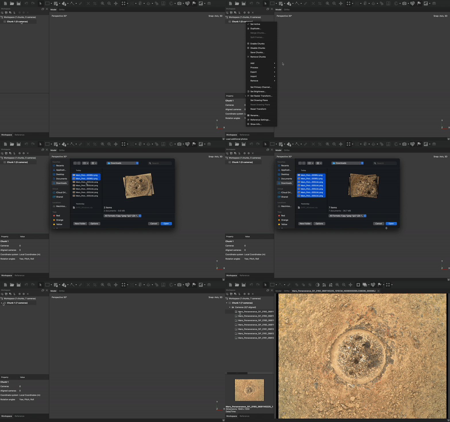Figure 2 Tips & Tricks: Images can also be imported to Metashape by simply dragging and dropping them into “Chunk 1” from another window.

Please note that Metashape does not currently offer an auto-save feature and thus the regular use of the “Ctrl+S” keyboard shortcut is highly encouraged.

2. Masking Images

Masking allows users to identify the image pixels associated with unwanted features. This feature is extremely useful since parts of Perseverance Rover often sneak their way into the camera’s line of view, and most images contain a black border around them.

Metashape allows users to either import a mask or mask an image manually. To import a mask, select all the images within Chunk 1, and double-click the selection to bring up the “import masks” tab. Set the following image parameters on the proceeding pop-up window: “Method: From File,” “Operation: Replacement,” “Filename template: SIF_mask_.jpg,” “Apply to: Selected Cameras,” and select “OK” after navigating to the downloaded folder’s directory. (see Figure 3) These settings will add a premade mask to all the selected images. A white outline indicating the masked features should now appear on each image.

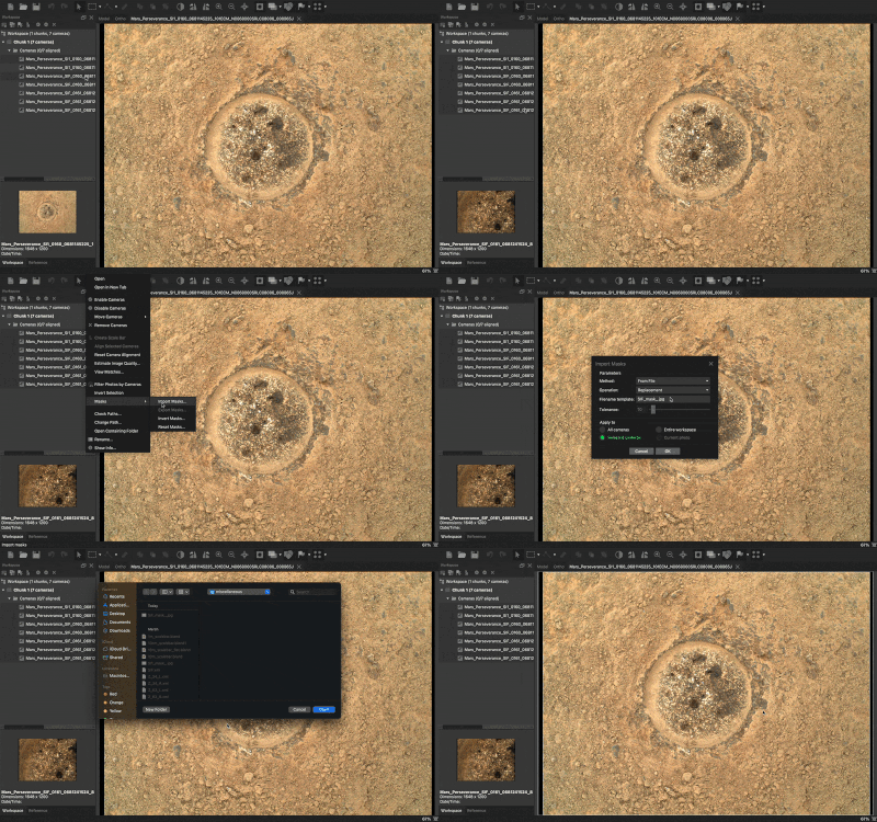Figure 3 Tips & Tricks: Files may not appear visible or selectable when navigating to the mask’s directory as the software was already informed of the file’s name and how to import it within the previous step. Thus, clicking “OK” once within the file’s directory is enough for the software to find the mask itself. If an error occurs after clicking “OK,” make sure the file name matches the one within its home directory.

3. Adding Camera Calibration (Optional)

Structure from Motion software is largely dependent on supplied images and metadata (extra data) to create models. The most important metadata is what kind of camera captured the images. Metashape has a good way of guessing the right camera parameters, but the more information you can give it the better. The most important parameter is the camera’s focal length in pixels, millimeters, or 35mm equivalent. The focal length combined with the image’s number of pixels (which Metashape automatically gets in front of the images) gives you the camera’s field-of-view (FOV). The Mars 2020 WATSON camera has a FOV of about 30 degrees. Just by knowing that and doing a little trigonometry, you can calculate that WATSON’s focal length is about 3000 pixels. But you don’t need to do any math. Just change the type to “Pre-Calibrated” and put the focal-length value of pixels in Metashape’s “Camera Calibration” window. (see Figure 4) From just the images and that focal-length value, Metashape can adequately constrain the camera further. See Figure 4 for where to find those options.

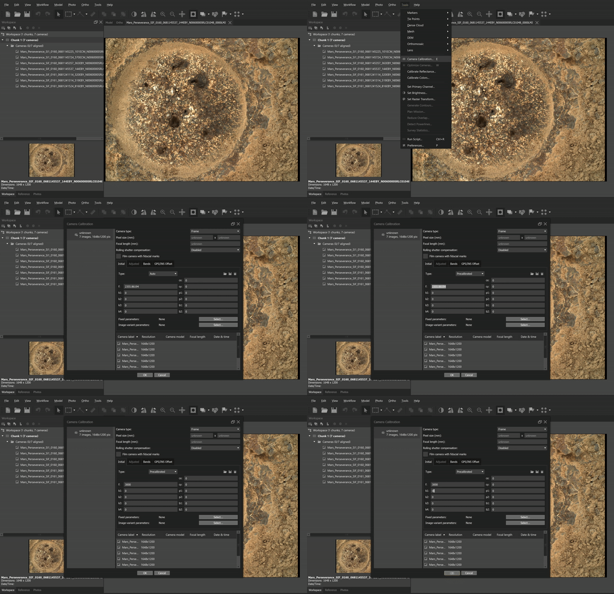Figure 4 Users are able to import camera positions to assist the software’s depth perception by going to “Tools” on the navigation bar, selecting “camera calibration,” and selecting the file icon on the pop-up menu to import data.

4. Aligning Photos

Agisoft Metashape converts 2D images into a 3D model by identifying shared features across multiple images. Metashape then uses these “key points” to estimate camera positions, generate depth maps, and determine the 3D shape. Under “Workflow” on the top menu bar, find “Align Photos,” and set the following specifications: set accuracy to “Highest;” turn on “generic pre-selection;” make sure “adaptive camera model fitting” and “exclude stationary tie points” are the only checkboxes enabled under “advanced;” and set the “key point limit” to zero as this will allow Metashape to find as many similarities across images as possible. (see Figure 5) All other default settings can remain unchanged.

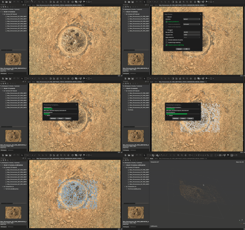Figure 5 In the Workflow tab, select the “Align Images” option and press “OK.” This action will establish a correlation between the images and determine their relative positions in three-dimensional space.

Several blue and grey points will now be projected onto each image. If these points are not visible, make sure “Show Points” is enabled by selecting the four-dot symbol on the main toolbar. Both types of points are correspondences found between images, but only the blue points are accurate enough to use.

Double-click on “Tie Points” in the workspace window to see the 3D point cloud. The “7” keyboard key will give a top-down centered view of the x-y axis projection; other navigation shortcuts are available by finding the “Predefined Views” tab within the drop-down menu under the top menu bar’s “Model” tab. Enabling the camera symbol on the main toolbar will display the rover’s camera positions with respect to the point cloud.

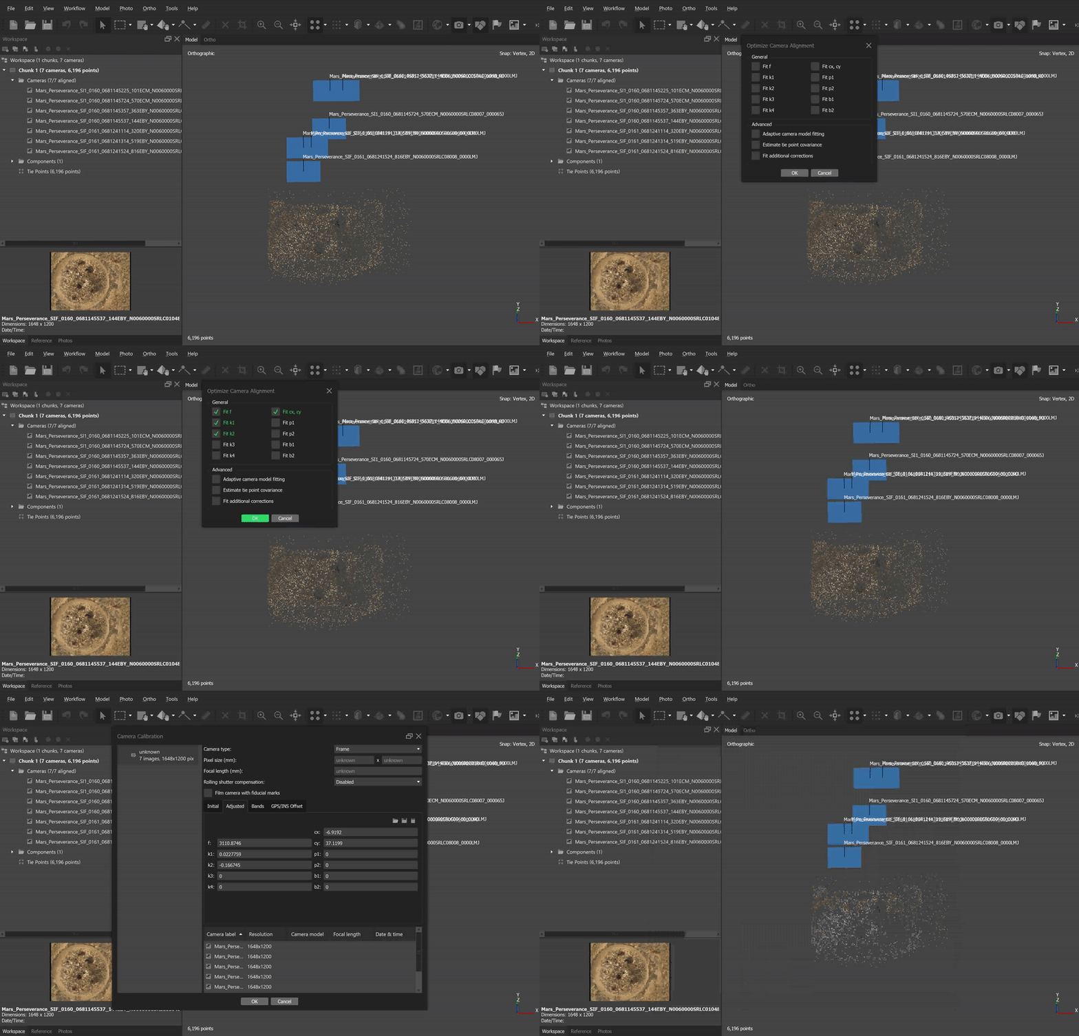Figure 6 (Optional) To reduce any potential alignment errors, find the “Optimize Camera Alignment” feature under the “Tools” drop-down menu located at the top menu bar. Check the first few boxes in the menu. It is also good to choose “Adaptive camera model fitting” under “Advanced” and select “OK.”

5. Generating a Mesh from Depth Maps

Now we turn this point cloud into a continuous 3D surface or mesh. Similar to a blank canvas, in 3D modeling, a “mesh” is considered to be the structural foundation onto which a model is projected. This process is possible by connecting points within the point cloud to form two-dimensional polygons within a three-dimensional plane.

Navigate to the “Build Mesh” feature under “Workflow” on the top menu bar, and set the following specifications: “Source Data: Depth Maps;” “Surface type: Arbitrary 3D;” “Quality: Ultra High;” “Depth filtering: Mild;” enable “interpolation;” and disable vertex color calculation to prevent difficulties when exporting the model. See Figure 7 for our recommended build mesh settings. Note that this step takes the most time, so feel free to let your computer run for a while (1-10 minutes depending on your computer’s power).

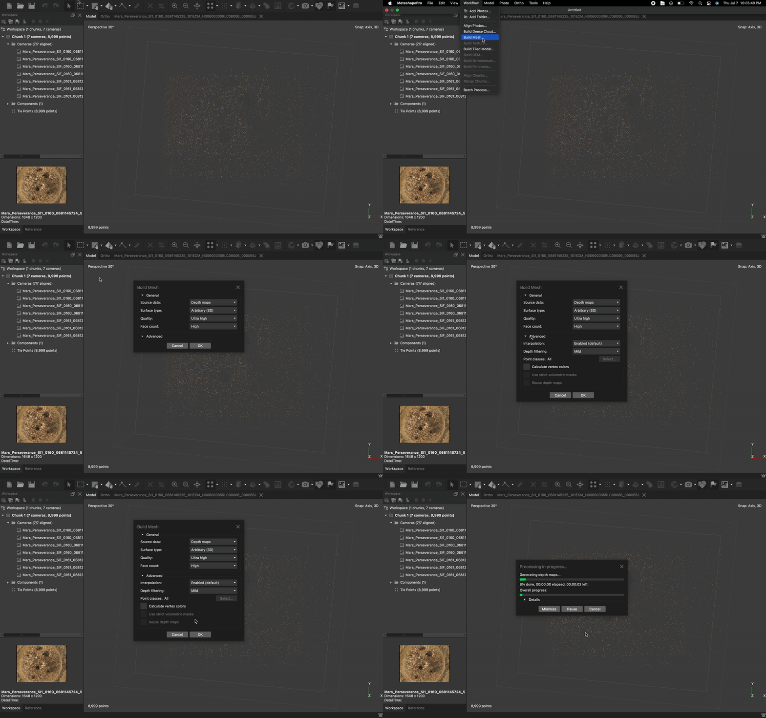Figure 7 When the images are aligned and optimized, choose the “Build Mesh” option in the “Workflow” menu. This will analyze the tie points to make the best continuous 3D model that it can.

To view the resulting mesh, exit Image View by selecting the “Model” tab. You may notice a box-like shape surrounding the generated point cloud and mesh. The area located within the box’s vertices is known as the model’s region. In cases where the point cloud displays a larger desired area than desired for the model, or if the model requires cropping, users are able to resize, rotate, and move the region to indicate the specific area from which a mesh should be generated.

Note, if there is an annoying white ball in the middle of your model, then go to the “Model” tab and under “Show/Hide” Items deselect “Show Trackball”.

6. Creating a Texture

If a mesh is analogous to a canvas, then a texture can be thought of as the design projected on to the canvas. This is the stage where the model will finally resemble our desired final product. To create a texture, find the “Build Texture” feature under “Workflow” along the main menu bar, and set the following specifications: “Texture Type: Diffuse Map;” “Source Data: Images;” “Mapping Mode: Generic;” “Blending Mode: Mosaic;” “Texture Size/Count:” choose 2048 or 4096 depending on the desired resolution. Models with higher texture quality can have larger file sizes and take more of your computer’s memory when loading them. Under “Advanced,” enable both hole-filling and ghost-filtering as seen in Figure 8.

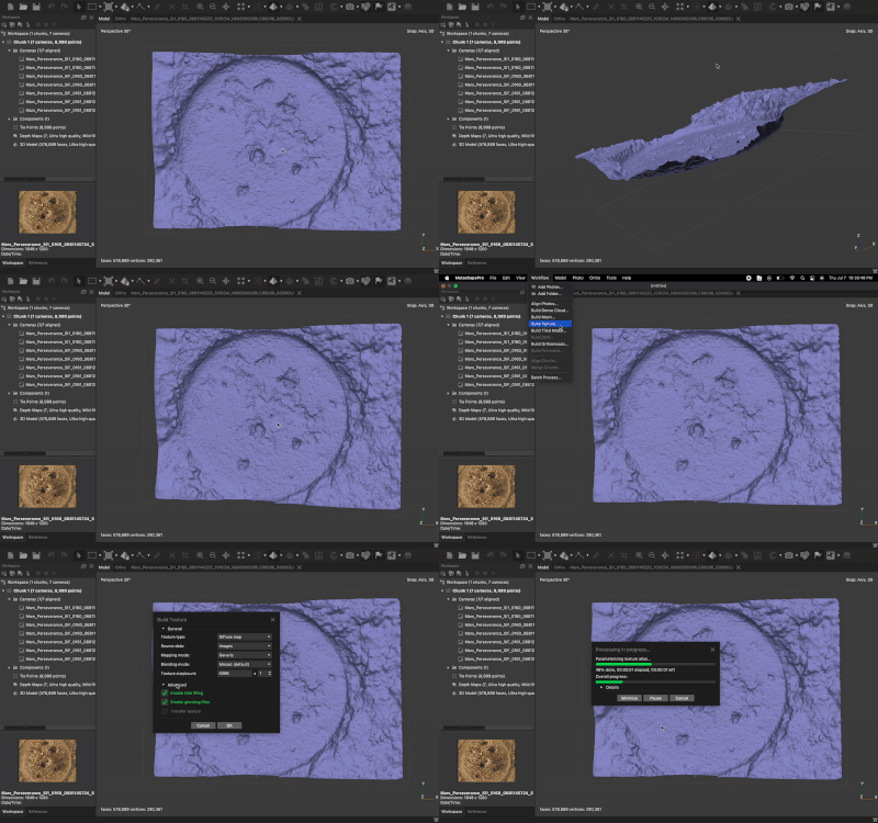Figure 8 Tips & Tricks: Texture sizes are optimized with texture sizes generated from multiples of 2: typically 1024, 2048, or 4096.

To view the resulting texture, switch the model view from either “Model Solid” or “Model Confidence” to “Model Textured.” (See Figure 9) Notice that features from the original WATSON images are now projected onto the corresponding region on the mesh.

7. Editing the Model

Agisoft Metashape offers many methods of editing models to make sure they meet the user’s expectations for the final product. If heavy shadows or unwanted features show up on the generated mesh, users can try either manually masking shadows within the original images under Chunk 1 or simply disabling problematic images altogether. Additionally, if the source images were taken under different lighting conditions, users can try calibrating colors and white balance under “Tools” along the main menu bar (see Figure 9). Regenerate the texture to see the changes. If the colors do not look better, then go back to the “Calibrate Colors” window and push “Reset” to return the images to their original colors.

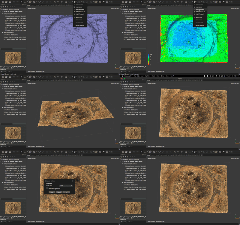Figure 9 Since some images can have different lighting, it often helps to white balance the images so that the images are more consistent. Find the “Calibrate Colors” option in the “Tools” menu, and click “Calibrate White Balance” and push “OK”.

8. Exporting the Model

To export the model, right-click the model’s name along the left navigation bar and select “Export Model…” in the resulting pop-up window. (see Figure 10)  When a 3D model is exported and downloaded as an OBJ file format, the system splits the model into three separate components: mesh, texture, and material. Each component is exported as its own individual file, allowing for greater flexibility and ease of inspection. The mesh file contains information about the geometry and shape of the model, including its vertices, edges, and faces. The texture file holds the information about the color and appearance of the model’s surface, such as its patterns and images. Finally, the material file contains information about the physical properties of the model, such as its reflectivity, transparency, and surface roughness. By having these components separated, it becomes easier to examine and edit each component independently, providing greater control and precision in the modeling process.

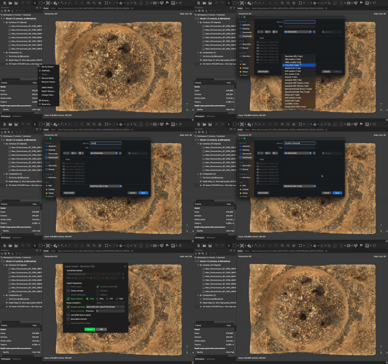Figure 10 Exporting the model as an obj. file allows for the model to be more accessible as those who download it will be able to directly investigate the mesh, texture, and material text file.

Part III: Uploading a model to Sketchfab

Science isn’t truly completed until it’s communicated. To ensure our models reach the largest audience possible, we turn to Sketchfab, a leading 3D model-sharing platform containing a vast community of 3D artists from every background.

1. Importing a Model

Upon creating a Sketchfab account, navigate to the “Upload” icon on the site’s toolbar. On the proceeding screen, click the “browse” button and navigate to the directory on your device containing the model’s saved obj, JPEG, and HTML files that were downloaded from Agisoft Metashape earlier. (see Figure 10)

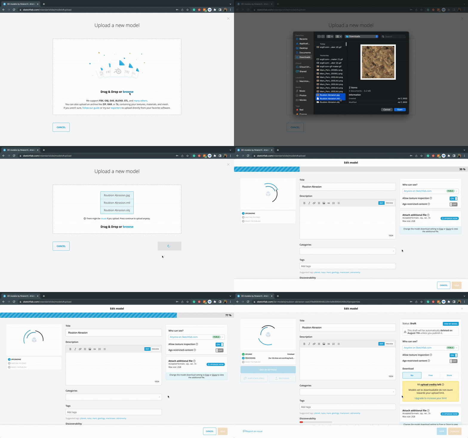Figure 10 Tips & Tricks: Files can also be imported by simply dragging and dropping them into Sketchfab’s Upload page from another window.

2. Setting up the Model for Display

Once fully loaded, enabling “texture inspection” and free downloads of the model provides the audience with more accessibility to the model.

Navigate to the “Edit 3D Settings” page where final edits to the model can be made before publishing. Select the “reset orientation” symbol under the “General” drop-down menu and click the right “x” arrow once under “straighten model.” (see Figure 11) These settings provide the uploaded model with a proper orientation reference when viewed. To properly display the model on Sketchfab, start by adjusting the shading settings to “shadeless.” Next, change the field of view to 30 degrees and turn off the “vertex color” option. After making these changes, don’t forget to save the file. Sketchfab’s “post-processing filters” also allow users to edit aspects of the model such as sharpness and color balance to fix any irregularities that may have resulted from lighting differences in the original image sets. (see Figure 11)

Finally, to set the model’s thumbnail on Sketchfab, simply click “save view” while the model is in the desired position. Once all these steps have been completed, select “publish” and congratulate yourself on your contribution to the Mars Sample Return Mission!

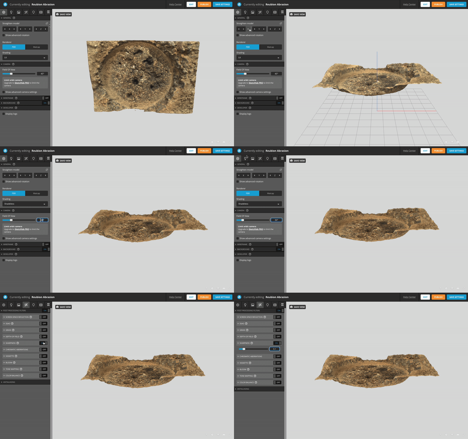Figure 11 Tips & Tricks: If the model’s texture isn’t visible when uploaded to another platform, whether given an error or presented with a monochromatic version of the model, try downloading the model as a glb file. Downloading the model as a glb file will automatically snap the model’s texture onto its mesh. Alternatively, try turning off “Vertex color” on the Sketchfab “3D Settings” page, or the base color under “materials.”

Generating models like these is a photogrammetric process called Structure from Motion (or SfM). SfM compiles several images taken from different angles of the same scene and semi-automatically produces a 3D product. Software applications for SfM, such as Agisoft Metashape which we use for these models, are readily available and continue to grow in performance and accessibility. SfM models have grown in popularity through 3D modeling communities, like Sketchfab – the social media viewer and repository for 3D models used in the above models, making it easier for developers to share their work with all.

To learn more about how these models are used to visualize the Mars Sample Return mission at the Rochette sample site, the extraction of samples, 3D modeling of the martian terrain, and how to access images and data directly from the Perseverance Rover, please visit our own Mastcam-Z blog to browse a vast collection of news and updates!

Note: All original image files for this blog can be downloaded from this Google Drive link.

Additional blog inspiration:

• Introduction to photogrammetry: How to use Metashape for Mac (in Japanese)
• Photogrammetry tutorial 11: How to handle a project in Agisoft Metashape (Photoscan)
• Creating 3D Models with Agisoft Metashape
• Agisoft Help Desk: 3D model reconstruction